Learning From Data——拟合sin曲线
这次的作业是用神经网络来拟合sin曲线。通过实践更能感受到ReLU以及sigmoid,tanh激活函数的区别。
作业中已经将整体框架写好,好让我们能专注于算法部分。比较复杂的部分是向量化,因为自己的博客定义的这个矩阵的形式可能是多样的,但是最后的结果肯定是一致的,以及需要传入的参数如何分配。
我选择传入的input为\(a^{(l)}\)以及\(a^{(l-1)}\),传入的gran_out为\(\sigma^{(l)}\)中除去乘\(g'(z)\)的部分。因为导数部分需要上一层的激活函数来决定。
在作业中定义W,a的方式和我定义\(\Sigma,a\)的方式正好相反,这是需要注意的地方。
这个神经网络包含4层:输入层,全连接层(1×80),ReLU层(80×80),输出层(80×1)。
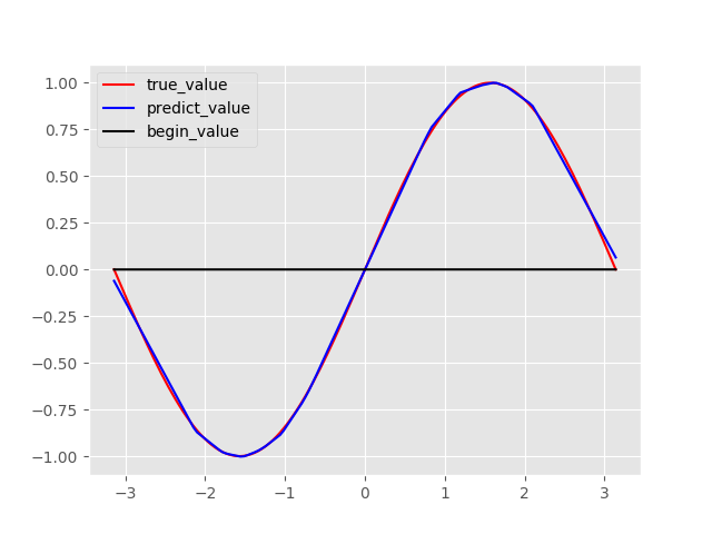
最后得到的拟合结果和loss曲线如下:
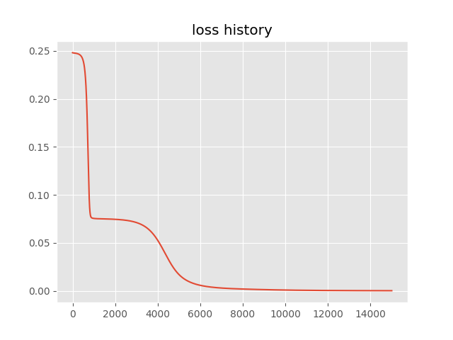
purelin:
loss history:
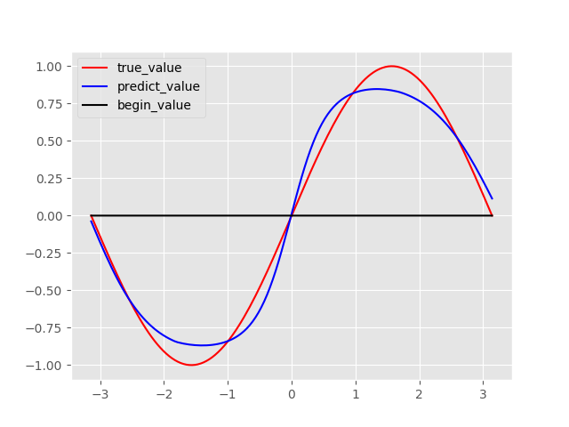
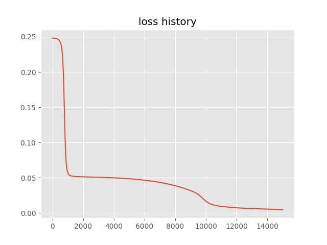
tanh:
loss history:
代码会在作业截止后上传。 1
2
3
4
5
6
7
8
9
10
11
12
13
14
15
16
17
18
19
20
21
22
23
24
25
26
27
28
29
30
31
32
33
34
35
36
37
38
39
40
41
42
43
44
45
46
47
48
49
50
51
52
53
54
55
56
57
58
59
60
61
62
63
64
65
66
67
68
69
70
71
72
73
74
75
76
77
78
79
80
81
82
83
84
85
86
87
88
89
90
91
92
93
94
95
96
97
98
99
100
101
102
103
104
105
106
107
108
109
110
111
112
113
114
115
116
117
118
119
120import numpy as np
import matplotlib.pyplot as plt
plt.style.use('ggplot')
x = np.linspace(-np.pi,np.pi,140).reshape(140,-1)
y = np.sin(x)
lr = 0.02 #set learning rate
def sigmoid(x):
return 1/(np.ones_like(x)+np.exp(-x))
def tanh(x):
return (np.exp(x) - np.exp(-x))/(np.exp(x) + np.exp(-x))
def mean_square_loss(y_pre,y_true): #define loss
loss = np.power(y_pre - y_true, 2).mean()*0.5
loss_grad = (y_pre-y_true)/y_pre.shape[0]
return loss , loss_grad # return loss and loss_grad
class ReLU(): # ReLu layer
def __init__(self):
pass
def forward(self,input):
unit_num = input.shape[1]
# check if the ReLU is initialized.
if not hasattr(self, 'W'):
self.W = np.random.randn(unit_num,unit_num)*1e-2
self.b = np.zeros((1,unit_num))
temp = input.dot(self.W) + self.b.repeat(input.shape[0]).reshape(self.W.shape[1],input.shape[0]).T
return np.where(temp>0,temp,0)
def backward(self,input,grad_out):
a_lm1 = input[0]
a_l = input[1]
derivative = np.where(a_l>0,1,0)
sample_num = a_lm1.shape[0]
delt_W = a_lm1.T.dot(grad_out*derivative)/sample_num
delt_b = np.ones((1,sample_num)).dot(grad_out*derivative)/sample_num
to_back = (grad_out*derivative).dot(self.W.T)
self.W -= lr * delt_W
self.b -= lr * delt_b
return to_back
class FC():
def __init__(self,input_dim,output_dim): # initilize weights
self.W = np.random.randn(input_dim,output_dim)*1e-2
self.b = np.zeros((1,output_dim))
def forward(self,input):
#purelin
#return input.dot(self.W) + self.b.repeat(input.shape[0]).reshape(self.W.shape[1],input.shape[0]).T
#tanh
return tanh(input.dot(self.W) + self.b.repeat(input.shape[0]).reshape(self.W.shape[1],input.shape[0]).T)
# backpropagation,update weights in this step
def backward(self,input,grad_out):
a_lm1 = input[0]
a_l = input[1]
sample_num = a_lm1.shape[0]
#purelin
'''delt_W = a_lm1.T.dot(grad_out)/sample_num
delt_b = np.ones((1,sample_num)).dot(grad_out)/sample_num
to_back = grad_out.dot(self.W.T)'''
#tanh
delt_W = a_lm1.T.dot(grad_out*(1-np.power(a_l,2)))/sample_num
delt_b = np.ones((1,sample_num)).dot(grad_out*(1-np.power(a_l,2)))/sample_num
to_back = (grad_out*(1-np.power(a_l,2))).dot(self.W.T)
self.W -= lr * delt_W
self.b -= lr * delt_b
return to_back
# bulid the network
layer1 = FC(1,80)
ac1 = ReLU()
out_layer = FC(80,1)
# count steps and save loss history
loss = 1
step = 0
l= []
while loss >= 1e-4 and step < 15000: # training
# forward input x , through the network and get y_pre and loss_grad
# To get a[l]
a = [x]
a.append(layer1.forward(a[0]))
a.append(ac1.forward(a[1]))
a.append(out_layer.forward(a[2]))
#backward # backpropagation , update weights through loss_grad
#sigma and a[l-1] is what the backpropagation needs. If you want get the derivative, the a[l] is also needed.
sigma = out_layer.backward([a[2],a[3]],a[3] - y)
sigma = ac1.backward([a[1],a[2]],sigma)
sigma = layer1.backward([a[0],a[1]],sigma)
#This step is for plotting the initial line.
if step == 0:
y_start = a[3]
step += 1
loss = mean_square_loss(a[3],y)[0]
l.append(loss)
#print("step:",step,loss)
y_pre = a[3]
# after training , plot the results
plt.plot(x,y,c='r',label='true_value')
plt.plot(x,y_pre,c='b',label='predict_value')
plt.plot(x,y_start,c='black',label='begin_value')
plt.legend()
plt.savefig('1.png')
plt.figure()
plt.plot(np.arange(0,len(l)), l )
plt.title('loss history')
# save the loss history.
plt.savefig('loss_t.png')