机器学习——(基石)作业3
总共20道题目。
1. Consider a noisy target \(y = {\bf w}_f^T{\bf x} + \epsilon\), where \(\mathbf{x} \in \mathbb{R}^d\) (with the added coordinate \(x_0=1\)), \(y\in\mathbb{R}\), \(\mathbf{w}_f\) is an unknown vector, and \(\epsilon\) is a noise term with zero mean and \(\sigma^2\) variance. Assume \(\epsilon\) is independent of \({\bf x}\) and of all other \(\epsilon\)'s. If linear regression is carried out using a training data set \(\mathcal{D} = \{(\mathbf{x}_1, y_1), \ldots, ({\bf x}_N, y_N)\}\), and outputs the parameter vector \(\mathbf{w}_{\rm lin}\), it can be shown that the expected in-sample error \(E_{\rm in}\) with respect to \(\mathcal{D}\) is given by: \[ \mathbb{E}_{\mathcal{D} }[E_{\rm in}(\mathbf{w}_{\rm lin})] = \sigma^2\left(1 - \frac{d + 1}{N}\right) \] For \(\sigma = 0.1\) and \(d = 8\), which among the following choices is the smallest number of examples \(N\) that will result in an expected \(E_{\rm in}\) greater than 0.008?
10
25
100
500
1000
这道题目中,已经给出了\(E_{in}\)的期望值如何计算,只需要将\(\sigma = 0.1,d = 8\)带入上式即可,算出来的是\(N = 45\)的时候,\(E_{in}\)的期望值为0.008,而为了使得期望值变得更大,\(N\)的值也要变得更大,因此上面选项中最小的大于45的\(N\)是100,选c(Note:Greater意思是更大,而不是更好).
2. Recall that we have introduced the hat matrix \(\mathrm{H} = \mathrm{X}(\mathrm{X}^T\mathrm{X})^{-1}\mathrm{X}^T\) in class, where \(\mathrm{X} \in \mathbb{R}^{N\times (d+1)}\) containing \(N\) examples with \(d\) features. Assume \(\mathrm{X}^T\mathrm{X}\) is invertible and \(N > d+1\), which statement of \(\mathrm{H}\) is true?
none of the other choices
\(\mathrm{H}^{1126} = \mathrm{H}\)
\((d+1)\) eigenvalues of \(\mathrm{H}\) are bigger than 1.
\(N - (d+1)\) eigenvalues of \(\mathrm{H}\) are 1
\(\mathrm{H}\) is always invertible
从linear regression中,我们直到\(H\)矩阵的作用是在\(X\)空间做\(Y\)的投影,来得到\(Y'\),而投影一次与投影10次没什么太大区别,因此b是正确的。\(H\)的自由度是\(N - (d+1)\),而它的特征值应该是有(N - d+1)个不为0,而且特征值也不是一定的,只是与特征向量成比例,因此c,d是不对的。
3. Which of the following is an upper bound of \([[sign(w^Tx)≠y]]\) for \(y \in \{-1, +1\}\)?
\(err(W) = \frac 1 2 e ^{(-yW^TX)}\)
\(err(W) = [W^TX \geq y]\)
\(err(W) = max(0,1 - yW^TX)\)
\(err(W) = max(0, -yW^TX)\)
none of the other choices
这个题目最直观的看法依然是画图,a-red,b-blue,c-yellow,d-green,\([sign(W^TX) \neq
y]\)-black,按照上面的颜色画图如下: 当y = 1 时: 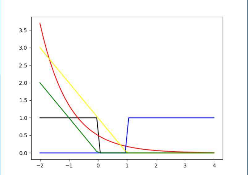 当 y = -1时:
 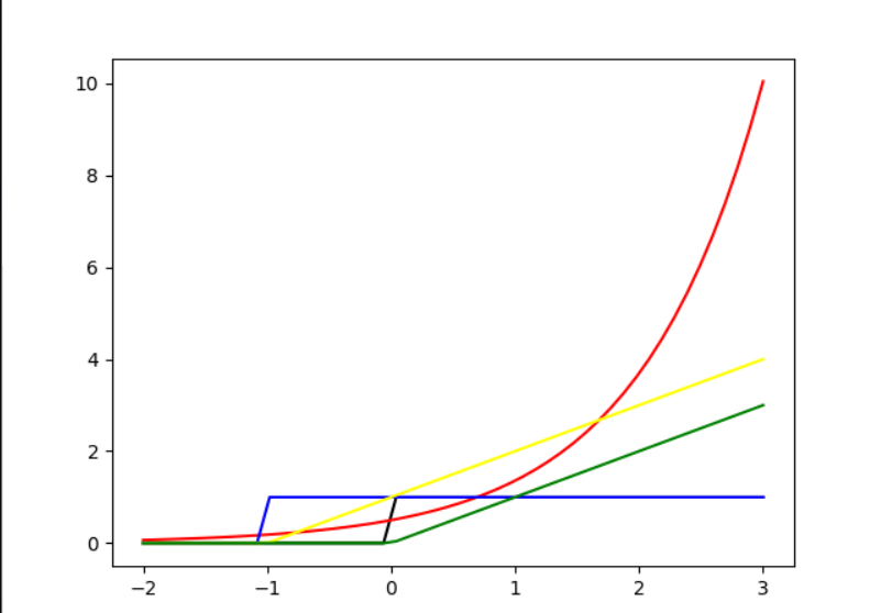 从上面的图中我们可以很直观看到只有yellow线是符合的,因此这个题目答案为c.
4. Which of the following is a differentiable function of \(\mathbf{w}\) everywhere?
\(err(W) = \frac 1 2 e ^{(-yW^TX)}\)
\(err(W) = [W^TX \geq y]\)
\(err(W) = max(0,1 - yW^TX)\)
\(err(W) = max(0, -yW^TX)\)
none of the other choices
differentiable function 意思是可微函数。所以很明显答案是a.
5. When using SGD on the following error functions and `ignoring' some singular points that are not differentiable, which of the following error function results in PLA?
\(err(W) = \frac 1 2 e ^{(-yW^TX)}\)
\(err(W) = [W^TX \geq y]\)
\(err(W) = max(0,1 - yW^TX)\)
\(err(W) = max(0, -yW^TX)\)
none of the other choices
PLA更新策略: \[ W_{n+1} = W_{n} + yX \] 使用SGD,也就是随机选择一个样本求\(err(W)\)的导数来更新。对于梯度下降中,对于下一步的做法是: \[ W_{n+1} = W_{n} - \alpha \frac {d_{err{W} } }{d_W} \] 其中\(\alpha\)是学习率,这道题目中应该为1.
因此主要是要求得导数。实际上,我们从上面的题目中可以轻易的看出,对于 a,b一定是不正确的,而c,d的导数是一样的:\(\frac {d_{err{W} } }{d_W} = -yX\),因此就更新的步骤来说,它们两个都是合适的。
但是我们不能都选上,要注意PLA算法做更新的时候是找到错误的点,如果点是正确的,我们则不应该更新。而c选项是PLA的Upper bound,从上面题目的图中也可以看到,如果\(y = -1,W^TX \in [-1,1]\)之间PLA是不会更新的,而c在这个时候依然会选择更新。所以这个题目的正确答案是d.
For Questions 6-10, consider a function \(E(u,v) = e^u + e^{2v} + e^{uv} + u^2 - 2 u v + 2 v^2 - 3 u - 2 v\).
6. What is the gradient \(\nabla E(u, v)\) around \((u, v)=(0, 0)\)?
\((0,-2)\)
none of the other choices
\((-3,1)\)
\((3,-1)\)
\((-2,0)\)
这道题目不算难。 \(\nabla E(u,v) = (e^u+ve^{uv}+2u - 2v - 3, 2e^{2v}+ue^{uv}-2u +4v - 2)\),代入\((0,0)\)得到\((-2,0)\),答案为e.
7. In class, we have taught that the update rule of the gradient descent algorithm is \((u_{t+1}, v_{t+1}) = (u_t, v_t) - \eta \nabla E(u_t, v_t)\). Please start from \((u_0, v_0) = (0, 0)\), and fix \(\eta=0.01\). What is \(E(u_{5}, v_{5})\) after five updates?
4.904
3.277
2.825
2.361
1.436
这个题目虽然迭代次数不多,但是因为有\(\exp\)函数计算,还是比较复杂的。因此我编写梯度下降的程序来计算这道题目。
函数gradient_decent要传入4个参数:start开始值,get_gradicent 一个计算梯度的函数,eta学习率,i_times为迭代次数。
其他的函数包括计算梯度,更新W(update),以及计算\(err\),程序代码如下: 1
2
3
4
5
6
7
8
9
10
11
12
13
14
15
16
17
18
19
20
21
22
23import math
import copy
def get_gradient(para):
return [math.exp(para[0])+para[1]*math.exp(para[0]*para[1])+2*para[0]-2*para[1]-3,2*math.exp(2*para[1])+para[0]*math.exp(para[0]*para[1] )- 2*para[0]+4*para[1]-2]
def gradient_decent(start,get_gradient,eta,i_times):
last = copy.deepcopy(start)
while(i_times>0):
i_times-=1
update(last,get_gradient(last),eta)
return last
def update(last,gradient,eta):
for i in range(len(last)):
last[i] = last[i] - eta * gradient[i]
return last
def Ein(para):
u = para[0]
v = para[1]
return math.exp(u)+math.exp(2*v)+ math.exp(u*v)+math.pow(u,2)-2*u*v+2*math.pow(v,2)-3*u - 2*v
if __name__ == "__main__":
print(gradient_decent([0,0],get_gradient,0.01,5))
print(Ein(gradient_decent([0,0],get_gradient,0.01,5)))
最后输出: 1
2[0.09413996302028127, 0.0017891105951028273]
2.8250003566832635
8. Continuing from Question 7. If we approximate the \(E(u + \Delta u, v + \Delta v)\) by \(\hat{E}_2(\Delta u, \Delta v)\), where \(\hat{E}_2\) is the second-order Taylor's expansion of \(E\) around \((u,v)\). Suppose $2(u, v) = b{uu} (u)^2 + b_{vv} (v)^2 + b_{uv} (u)(v) + b_u u + b_v v + b $, What are the values of \((b_{uu}, b_{vv}, b_{uv}, b_u, b_v, b)\) around \((u, v) = (0, 0)\)?
none of the other choices
\((3,8,-1,-2,0,3)\)
\((3,8,-0.5,-1,-2,0)\)
\((1.5,4,-0.5,-1,-2,0)\)
\((1.5,4,-1,-2,0,3)\)
这个题目不算难,实际上是一个多维函数的二阶泰勒展开,而\(b{_uu}\)则是对\(u\)求二阶偏导再除以\(2!\)。只要一项项计算上面的值就可以了。 \(b_{uu} = 3,b_{vv} = 8,b_{uv} = -1,b_{u} = -2,b_{v} = 0,b = 3\),二元泰勒展开因此答案是e.
9. Continue from Question 8 and denote the Hessian matrix to be \(\nabla^2 E(u, v)\), and assume that the Hessian matrix is positive definite. What is the optimal \((\Delta u, \Delta v)\) to minimize \(\hat{E}_2(\Delta u, \Delta v)\)? (The direction is called the Newton Direction.)
\(+(\nabla^2E(u,v))^{-1}\nabla E(u,v)\)
\(-(\nabla^2E(u,v))^{-1}\nabla E(u,v)\)
none of the other choices
\(+\nabla ^2 E(u,v) \nabla E(u,v)\)
\(-\nabla ^2 E(u,v) \nabla E(u,v)\)
其实这个题目我不是很清楚。这其中涉及到了海森矩阵以及牛顿方向。通过简单的了解,如果一个点的梯度为0向量,而且在该点的海森矩阵为正定矩阵,那么该点为极小值点。题目中说明了海森矩阵为正定矩阵,因此找这个极值点,如果不知道牛顿方向,我就会按照梯度下降的来。而查阅了牛顿方向之后,牛顿方向就是e选项。所以选择b.
当然,这个题目实际上就是搜出来的答案,真正想要理解需要更加深入地去看线性代数。
10. Use the Newton direction (without ) for updating and start from \((u_0, v_0) = (0, 0)\). What is \(E(u_{5}, v_{5})\) after five updates?
4.904
3.277
2.825
2.361
1.436
这道题目,当然我还是想借助程序来完成,不过这次的程序相比之前会更麻烦一点。因为之前设置好了接口,也就是在梯度下降的时候传入求得梯度的函数,因此这里我们只需要写出计算
\(\nabla ^2 E(u,v) \nabla
E(u,v)\)的函数: 1
2
3
4
5
6
7def Newton_direction(para):
u = para[0]
v = para[1]
hs = [[math.exp(u)+math.pow(v,2)*math.exp(u*v)+2,math.exp(u*v)+v*u*math.exp(u*v)-2],
[math.exp(u*v)+v*u*math.exp(u*v)-2,4*math.exp(2*v)+math.pow(u,2)*math.exp(u*v)+4]]
m = mat(hs)
return (m.I*mat([get_gradient([u,v])]).T).T.tolist()[0]1
print(Ein(gradient_decent([0,0],Newton_direction,1,5)))
2.360823345643139 因此答案选d.
11. Consider six inputs \(\mathbf{x}_1 = (1, 1)\), \(\mathbf{x}_2 = (1, -1)\), \(\mathbf{x}_3 = (-1, -1)\), \(\mathbf{x}_4 = (-1, 1)\), \(\mathbf{x}_5 = (0, 0)\), \(\mathbf{x}_6 = (1, 0)\). What is the biggest subset of those input vectors that can be shattered by the union of quadratic, linear, or constant hypotheses of \(\mathbf{x}\)?
\(\mathbf{x}_1,\mathbf{x}_2,\mathbf{x}_3\)
\(\mathbf{x}_1,\mathbf{x}_2,\mathbf{x}_3,\mathbf{x}_4,\mathbf{x}_5,\mathbf{x}_6\)
\(\mathbf{x}_1,\mathbf{x}_2,\mathbf{x}_3,\mathbf{x}_4\)
\(\mathbf{x}_1,\mathbf{x}_3\)
\(\mathbf{x}_1,\mathbf{x}_2,\mathbf{x}_3,\mathbf{x}_4,\mathbf{x}_5\)
首先,我们可以看到特征量的个数是2(\(d=2\)),而由前面的推导可以知道,最高次为2次时候,它可以组成的新的特征值的个数为5,而它的vc dimension是小于等于6的.一种可行的办法是将x空间投影到z空间以后,用线性的办法来shatter这6个点,再返回看原来的x组合而成的特征是否能够满足这6个特征量。但是实际上这还是复杂的。也可以利用梯度下降,跑程序来对上述选项来进行排除。具体答案是多少还需要进一步进行排除。这个答案是b.可以shatter6个点.
12. Assume that a transformer peeks the data and decides the following transform \(\boldsymbol{\Phi}\) "intelligently" from the data of size \(N\). The transform maps \(\mathbf{x} \in \mathbb{R}^d\) to \(\mathbf{z} \in \mathbb{R}^N\), where \[ (\boldsymbol{\Phi}(\mathbf{x}))_n = z_n = \left[\left[ \mathbf{x} = \mathbf{x}_n \right]\right] \] Consider a learning algorithm that performs PLA after the feature transform.Assume that all \(\mathbf{x}_n\) are different, \(30%\) of the \(y_n\)'s are positive, and \(sign(0)=+1\). Then, estimate the \(E_{out}\) of the algorithm with a test set with all its input vectors \(\mathbf{x}\) different from those training \(\mathbf{x}_n\)'s and \(30%\) of its output labels \(y\) to be positive. Which of the following is not true?
PLA will halt after enough iterations.
\(E_{out} = 0.7\)
\(E_{in} = 0.7\)
All \(\mathbf{Z}_n\)'s are orthogonal to each other.
The transformed data set is always linearly separable in the \(\mathcal{Z}\) space.
要明白这个题目首先要读懂题意。 题目中对原来的向量进行了特征转换,原来向量为d维,新的向量为N维,每一个样本对应的新的Z向量是 \([ [[x_i = x_1]], [[x_i = x_2]],...,[[x_i = x_n]]]^T\),题目中已经告知,\(X_n\)是各不相同的,因此我们可以直到\(Z\)向量会类似于:\([1,0,...,0]^T,[0,1,...,0]^T,...,[0,0,...,1]\).在这样的样本上进行PLA算法。我们可以知道这种情况是最好的情况,是可以被shatter的,PLA一定会停止,而且他们是互相正交的。因此答案就在b,c中选择。而既然PLA会停止说明找到了最小的\(E_{in}\),此时\(E_{in}\)为0.因此答案选c.
至于c为何是正确的,首先,因为测试集的样本与原来的训练集样本也没有一致的,因此他们得到的转换后的z向量为n维0向量.而题目中说明了\(sign(0)=+1\),因此它会将所有的测试样本都判别为positive,而实际上只有30%为positive,因此测试得到的\(E_{out}\)为70%.
For Questions 13-15, consider the target function: \[ f(x_1, x_2) = \mbox{sign}(x_1^2 + x_2^2 - 0.6) \]
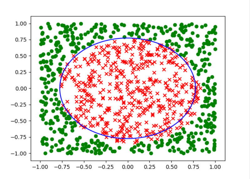
13. Generate a training set of N = 1000N=1000 points on \(X=[−1,1]\) with uniform probability of picking each \(\mathbf{x} \in \mathcal{X}\). Generate simulated noise by flipping the sign of the output in a random \(10\%\) subset of the generated training set.
Carry out Linear Regression without transformation, i.e., with feature vector: \[ (1,x_1,x_2) \]
to find the weight \(\mathbf{w}_{\rm lin}\), and use \(\mathbf{w}_{\rm lin}\) directly for classification. What is the closest value to the classification \((0/1)\) in-sample error (\(E_{\rm in}\))? Run the experiment \(1000\) times and take the average \(E_{\rm in}\) in order to reduce variation in your results.
0.1
0.3
0.5
0.7
0.9
这次作业与之前不一样了,很早就遇到编程题目了,而且前面有几道题目虽然不是编程题目,我也依然是用程序计算出来的。
这个题目想要用程序解答其实也不是非常难。在这里我使用的是一步求法,而不是梯度下降那样迭代。首先是要生成数据:
1
2
3
4
5
6
7def make_data():
result = []
for i in range(1000):
x1 = random.random()*2-1
x2 = random.random()*2-1
result.append([x1,x2,sign(pow(x1,2)+pow(x2,2)-0.6)])
return result
为了检查做的数据是否正确,对生成的数据进行了可视化(因为输出长宽比例不同,所以这个圆看上去不是正圆):
1
2
3
4
5
6
7
8
9
10
11
12
13
14
15
16
17
18
19
20
21
22
23
24def visualize(data,W=[]):
nx = []
ny = []
ox = []
oy = []
for i in range(len(data)):
if data[i][-1] == -1:
nx.append(data[i][1])
ny.append(data[i][2])
else:
ox.append(data[i][1])
oy.append(data[i][2])
plt.scatter(nx,ny,marker="x",c="r")
plt.scatter(ox,oy,marker="o",c="g")
theta = np.linspace(0, 2 * np.pi, 800)
x, y = np.cos(theta) * 0.77459666924148, np.sin(theta) * 0.77459666924148# sqrt 0.6
plt.plot(x, y, color='blue')
if len(W)!=0:
print(W)
x = np.linspace(-1, 1, 50)
y = -W[1] / W[2] * x - W[0] / W[2]
plt.plot(x, y, color="black")
plt.show()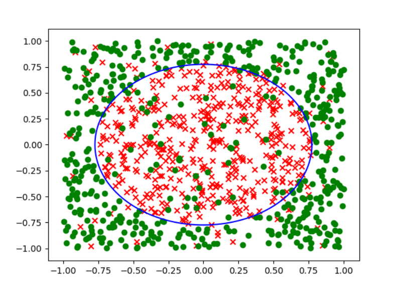
然后通过线性回归得到\(W =
(X^TX)^{-1}X^TY\): 1
2
3
4
5
6
7
8
9
10
11
12
13
14def linear_regression_one_step(data):
X_matrix = []
Y_matrix = []
for i in range(len(data)):
temp = []
for j in range(len(data[i])-1):
temp.append(data[i][j])
X_matrix.append(temp)
Y_matrix.append([data[i][-1]])
X = np.mat(X_matrix)
Y = np.mat(Y_matrix)
W = (X.T*X).I*X.T*Y
return W.T.tolist()[0]
最后通过分类计算\(E_{in}\):
1
2
3
4
5
6
7
8
9def Ein(data,W):
err_num = 0
for i in range(len(data)):
res = 0
for j in range(len(W)):
res += W[j]*data[i][j]
if sign(res) != data[i][-1]:
err_num+=1
return err_num
运行1000次取输出为:0.50614
因此答案选c.其实我们也可以想象得到这个错误率是接近0.5的,可视化的结果如下:
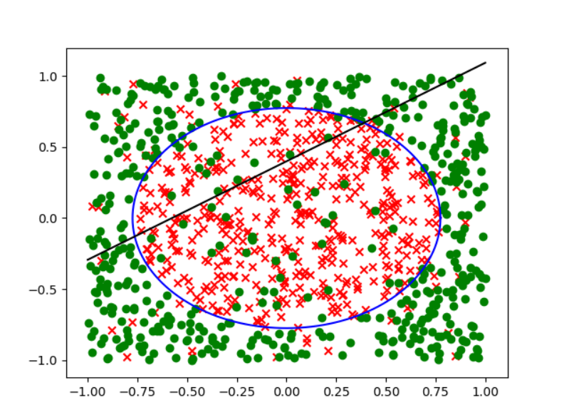
不管怎么画这条线,总会有接近一半的区域被分错.
14. Now, transform the training data into the following nonlinear feature vector:\((1,x_1,x_2,x_1x_2,x_1^2,x_2^2)\).Find the vector \(\tilde{\mathbf{w} }\) that corresponds to the solution of Linear Regression, and take it for classification. Which of the following hypotheses is closest to the one you find using Linear Regression on the transformed input? Closest here means agrees the most with your hypothesis (has the most probability of agreeing on a randomly selected point).
\(g(x_1,x_2) = sign(-1-1.5x_1+0.08x_2+0.13x_1x_2+0.05x_1^2+1.5x_2^2)\)
\(g(x_1,x_2) = sign(-1-1.5x_1+0.08x_2+0.13x_1x_2+0.05x_1^2+0.05x_2^2)\)
\(g(x_1,x_2) = sign(-1-0.05x_1+0.08x_2+0.13x_1x_2+1.5x_1^2+15x_2^2)\)
\(g(x_1,x_2) = sign(-1-0.05x_1+0.08x_2+0.13x_1x_2+1.5x_1^2+1.5x_2^2)\)
\(g(x_1,x_2) = sign(-1-0.05x_1+0.08x_2+0.13x_1x_2+15x_1^2+1.5x_2^2)\)
经过特征转换后进行线性回归,找到最相似的W向量。实际上,每次输出的向量不容易看出来他们的相似性,最好的办法就是从z空间转回去看实际的分类效果。
为了完成这道题目,需要添加一些新的函数。首先是一个特征转换的函数:
1
2
3
4
5
6
7
8
9
10
11
12
13def transform_data(data):
t_data = []
for i in range(len(data)):
temp = [1]
temp.append(data[i][1])
temp.append(data[i][2])
temp.append(data[i][1]*data[i][2])
temp.append(data[i][1]*data[i][1])
temp.append(data[i][2]*data[i][2])
temp.append(data[i][-1])
t_data.append(temp)
return t_data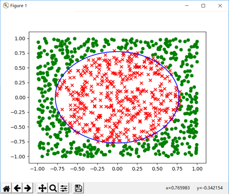
而其他几个选项按照a,b,c,d,e的顺序分别得到下面的分类效果: 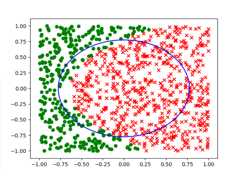
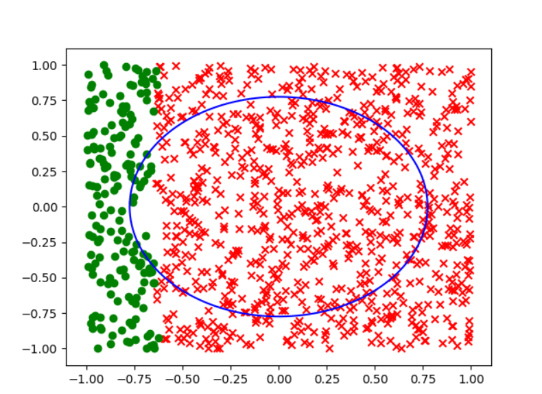
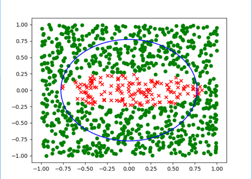
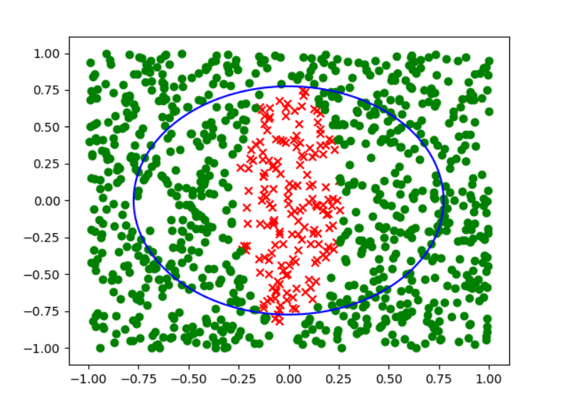
可以很明显的看出来,答案选择d.
15. Following Question 14, what is the closest value to the classification out-of-sample error \(E_{\rm out}\) of your hypothesis? Estimate it by generating a new set of 1000 points and adding noise as before. Average over 1000 runs to reduce the variation in your results.
0.1
0.3
0.5
0.7
0.9
这道题目需要来测量\(E_{out}\),并且要加上噪声。其实还是很简单的,只需要做简单的改动,来计算\(E_{out}\).
既然是\(E_{out}\),那就需要每次都重新生成数据,这就是和\(E_{in}\)的区别,再加个转换,除此之外是一样的,因此可以复用\(E_{in}\)函数: 1
2
3
4def Eout(W):
data = make_data()
t_data = transform_data(data)
return Ein(t_data,W)
然后运行1000次就可以了,最后得到的错误率:0.126856,答案选a.
For Questions 16-17, you will derive an algorithm for the multinomial (multiclass) logistic regression model. 16. For a \(K\)-class classification problem, we will denote the output space \(\mathcal{Y} = \{1, 2, \ldots, K\}\). The hypotheses considered by the model are indexed by a list of weight vectors \((\mathbf{w}_1, \mathbf{w}_2, \ldots, \mathbf{w}_K)\), each weight vector of length \(d+1\). Each list represents a hypothesis \[ h_y( X) = \frac {e^{W_y^TX} } {\sum _{k=1} ^{K} e^{W_k^TX} } \] that can be used to approximate the target distribution \(P(y|\mathbf{x})\)P. The model then seeks for the maximum likelihood solution over all such hypotheses.(Note:\(X\) = \(\mathbf{x}\))
For general \(K\), derive an \(E_{\text{in} }(\mathbf{w}_1, \cdots, \mathbf{w}_K)\) like page 11 of Lecture 10 slides by minimizing the negative log likelihood. What is the resulting \(E_{\text{in} }\)?
N {n = 1}^N ( {k=1} ^K (W_k^TX_n - W_{y_n}^TX_n))
N {n = 1}^N ({k=1} ^K W_k^TX_n - W_{y_n}^TX_n)
N {n = 1}^N ( ({k=1} ^K e{W_kTX_n}) - W_{y_n}^TX_n)
none of the other choices
N {n = 1}^N ( ({k=1} ^K e{W_kTX_n} - e{W_{y_n}TX_n}))
这是一个很有意思的概率的定义,它保证了分到各个分类的概率和加起来为1,而之前的假设是不能保证这个问题的。
对于\(E_{in}\)的处理,也是一致的。按照之前的想法来一步一步做。首先,计算出在该\(W\)的情况下,出现当前分类的概率,可以知道的是互相连乘,最后为了让他变成加法,以及最小化(而非最大化),需要加一个负号,忽略P(X=X_i)。
可以得到下面的过程:
\[ \prod_{i=n}^{N} \frac {e^{W_{y_n}^TX_{n} } } {\sum _{k=1} ^{K} e^{W_k^TX_n} } \]
\[ => -\sum_{n = 1}^N( \ln (e^{W_{y_n}^TX_n}) - \ln (\sum _{k = 1}^K e^{W_{k}^TX_n})) \]
\[ =>\sum _{n = 1}^N \left ( \ln (\sum _{k=1} ^K e^{W_k^TX_n} - W_{y_n}^TX_n)\right) \]
最后除以N,得到选项c.
17. For the \(E_{\text{in} }\) derived above, its gradient \(\nabla E_{\text{in} }\) can be represented by \(\left(\frac{\partial E_{\text{in} } }{\partial\mathbf{w}_1}, \frac{\partial E_{\text{in} } }{\partial\mathbf{w}_2}, \cdots, \frac{\partial E_{\text{in} } }{\partial\mathbf{w}_K}\right)\), write down \(\frac{\partial E_{\text{in} } }{\partial\mathbf{w}_i}\) .
N {n=1}^N ({i = 1} K(e{W_i^TX_n} - [[y_n=i]])X_n)
N _{n=1}^N ((h_i(x_n)-1)x_n)
none of the other choices
N _{n=1}^N ((h_i(x_n) - [[y_n=i]])X_n)
N {n=1}^N ( (i = 1)K(e{W_i^TX_n}-1)X_n)
这个题目就是对上面的题目的选择结果进行求导即可。虽然比较复杂,但是不算难。一步步算下来就成,正确答案是d.
For Questions 18-20, you will play with logistic regression. Please use the following set for training:
https://www.csie.ntu.edu.tw/~htlin/mooc/datasets/mlfound_algo/hw3_train.dat
and the following set for testing:
https://www.csie.ntu.edu.tw/~htlin/mooc/datasets/mlfound_algo/hw3_test.dat
18. Implement the fixed learning rate gradient descent algorithm for logistic regression. Run the algorithm with \(\eta = 0.001\) and \(T = 2000\). What is \(E_{out}(g)\) from your algorithm, evaluated using the \(0/1\) error on the test set?
0.475
0.412
0.322
0.220
0.103
19. Implement the fixed learning rate gradient descent algorithm for logistic regression. Run the algorithm with \(\eta = 0.01\) and \(T = 2000\). What is \(E_{out}(g)\) from your algorithm, evaluated using the \(0/1\) error on the test set?
0.475
0.412
0.322
0.220
0.103
20. Implement the fixed learning rate stochastic gradient descent algorithm for logistic regression. Instead of randomly choosing nn in each iteration, please simply pick the example with the cyclic order \(n = 1, 2, \ldots, N, 1, 2, \ldots\),Run the algorithm with \(\eta = 0.001\) and \(T = 2000\). What is \(E_{out}(g)\) from your algorithm, evaluated using the \(0/1\) error on the test set?
0.475
0.412
0.322
0.220
0.103
这3道题目,可以用一套方法做出来,可以引用第7题的程序中的梯度下降算法与13题程序中的对于\(E_{in}\)的估计。当然,对于之前代码的还需要进行一丝修改。
1
2
3
4
5
6
7
8
9
10
11
12
13
14
15
16
17
18
19
20
21
22
23
24
25
26
27
28
29
30
31
32
33
34
35
36
37
38
39
40
41
42
43
44
45
46
47
48
49
50
51
52
53
54import gradient_decent_7 as gd
import math
import numpy as np
import re
import _linear_regression_13 as lr
now = 0
def logistic(x):
return 1/(1+math.exp(-x))
def get_logistic_gradient(lastW,data):
W = np.mat([lastW]).T
X = []
for i in range(len(data)):
temp = data[i][0:-1]
temp.append(1)
X.append(np.mat([temp]).T)
gra = logistic(-data[0][-1]*(W.T*X[0])[0][0])*(-data[0][-1]*X[0])
for i in range(1,len(data)):
gra = gra + logistic(-data[i][-1]*(W.T*X[i])[0][0])*(-data[i][-1]*X[i])
#print(gra)
return ((1/len(data))*gra).T.tolist()[0]
def stochastic_gradient_init():
global now
now = 0
def stochastic_gradient(lastW,data):
global now
if now == len(data):
now = 0
W = np.mat([lastW]).T
temp = data[now][0:-1]
temp.append(1)
X = np.mat([temp]).T
gra = logistic(-data[now][-1]*(W.T*X)[0][0])*(-data[now][-1]*X)
now += 1
return gra.T.tolist()[0]
def readDataFrom(filename):
result = []
separator = re.compile('\t|\b| |\n')
with open(filename,'r') as f:
line = f.readline()[1:-1]
#print(line)
while line:
temp = separator.split(line)
#print(temp)
abc = [float(x) for x in temp]
#print(abc)
result.append(abc)
#print(result)
line = f.readline()[1:-1]
return result
还有一个readDataFrom不用多说,根据资料的输入形式进行适当调整。
最后在主函数中整合输出结果: 1
2
3
4
5
6
7
8
9
10
11
12
13
14
15
16
17if __name__ == "__main__":
data = readDataFrom("./hw3_train.dat")
start = [0 for x in range(0,len(data[0]))]
i_times = 2000
stochastic_gradient_init()
W1 = gd.gradient_decent(start,get_logistic_gradient,0.001,i_times,data)
W2 = gd.gradient_decent(start,get_logistic_gradient,0.01,i_times,data)
W3 = gd.gradient_decent(start,stochastic_gradient,0.001,i_times,data)
err1 = lr.Ein(data,W1)
err2 = lr.Ein(data,W2)
err3 = lr.Ein(data,W3)
out_data = readDataFrom("./hw3_test.dat")
err_out1 = lr.Ein(out_data,W1)
err_out2 = lr.Ein(out_data,W2)
err_out3 = lr.Ein(out_data,W3)
print("Ein:",err1,err1/len(data),err2,err2/len(data),err3,err3/len(data))
print("Eout:",err_out1,err_out1/len(out_data),err_out2,err_out2/len(out_data),err_out3,err_out3/len(out_data))
最后的结果,分别是3道题目的\({E_in}\)与\(E_{out}\).
1 | Ein: 430 0.43 204 0.204 427 0.427 |
因此我认为答案是a,d,a. 可以看到学习率过低的话可能会使得下降速度过慢,而且随机梯度下降的性能有时候不见得比普通的梯度下降差,但是速度却大大提高。
将迭代次数更新为10000,3个学习方法都取得了不错的效果,而步长大的性能反而不如之前,说明因为步长过大,它只能再最低点徘徊很难取得更低的位置,而步长小的依然没有达到极限:
1
2
Ein: 236 0.236 206 0.206 235 0.235
Eout: 779 0.25966666666666666 695 0.23166666666666666 776 0.25866666666666666
p.s.
1.python中的全局变量,list为引用,而赋值一个常数则会重新声明,为了避免歧义。因此想要改变全局变量的常数,需要添加关键词global。
2.牛顿方向与海森矩阵。